Exam solutions, Moed bet, 5766
These are only notes, not full answers.
All the questions can be answered in many ways!
Especially the ones in part B.
======================================================================
Part A, Question 1
==================
The rule: A B = C makes sense if A is m x n, B is n x p and C is m x p.
a) x=A\b => try to solve A x = b
Here A is 3 x 3 , b is 1 x 3
No solution
b) x=b/A => try to solve x A = b
Here A is 3 x 3 , b is 1 x 3
Solution with x = 1 x 3, i.e. a row vector.
If A has nonzero determinant this will be an exact solution
(If not, it may be an approximate solution, or one of an infinite
family of solutions)
c) x=A/b => try to solve x b = A
Here A is 3 x 3 , b is 1 x 3
Solution with x = 3 x 1, i.e. a column vector
Usually this will be an approximate solution (there are 9 equations
in 3 variables), if A has rank one it will be exact.
======================================================================
Part A, Question 2
==================
with(LinearAlgebra);
M:=<<t,sin(t),1>|<sin(t),t^2,cos(2*t)>|<1,cos(2*t),t^3>>;
int( Trace(Transpose(M).M) , t=0..2*Pi);
The answer is 128 pi^7/6 + 32 pi^5/5 + 8/3 pi^3/3 + 8 pi
======================================================================
Part A, Question 3
==================
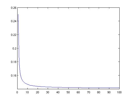
Here is a very elegant way to do it, there are many others:
a=zeros(1,100);
a(1)=1;
for n=2:100
a(n)=sum(a(1:n-1).*a(n-1:-1:1));
end
n=1:100;
plot( n , a.*n.^(3/2)./4.^n )
Here's the output:
 ======================================================================
Part A, Question 4
==================
Make an m-file newb.m with contents
function z=newb(x,y)
z=zeros(size(x));
for i=1:size(x,2)
if x(i)^2+y^2<1
z(i)=sin(2*x(i)*y)/(1+x(i)^2+y^2);
end
end
Then do dblquad(@newb,0,1,0,1) to get the answer 0.1458
======================================================================
Part A, Question 5
==================
The idea here is to follow how the root of x^2-3x+2-(i/3)sin(x)=0
changes as i changes.
When i=0 there are 2 roots: x=1 and x=2.
If we start from the x=1 root, then as i changes we see the root
decreases (gets close to zero). This is the b[i] sequence.
If we start from the x=2 root, then as i changes we see the root
increases (gets close to pi). This is the c[i] sequence.
======================================================================
Part B, Question 1
==================
restart; with(LinearAlgebra):
newb:=proc(a0,a1,b0,b1)
local t,x,x1,x2,v1,v2,kappa,gr1,gr2,ts,ts1;
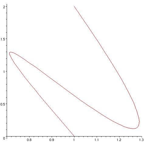
x:=Add( Add(a0,a1,(1-t)^3,3*t*(1-t)^2) , Add(b0,b1,t^3,3*t^2*(1-t)) );
x1:=x[1]; x2:=x[2];
gr1:=plot( [x1,x2,t=0..1] );
v1:=diff(x1,t); v2:=diff(x2,t);
kappa:=simplify( abs( diff(v1,t)*v2-diff(v2,t)*v1 ) / (v1^2+v2^2)^(3/2) );
gr2:=plot(kappa,t=0..1);
ts:=solve(kappa=0,t);
ts1:=NULL;
for i from 1 to nops(ts)
do if 0<evalf(op(i,ts)) and evalf(op(i,ts))<1
then ts1:=ts1,op(i,ts)
end if
end do;
return(print(gr1),kappa,print(gr2),ts1);
end proc;
Here is a set of results:
a0:=<1,2>; a1:=<2,-3>; b0:=<1,0>; b1:=<0,4>;
newb(a0,a1,b0,b1);
gives
======================================================================
Part A, Question 4
==================
Make an m-file newb.m with contents
function z=newb(x,y)
z=zeros(size(x));
for i=1:size(x,2)
if x(i)^2+y^2<1
z(i)=sin(2*x(i)*y)/(1+x(i)^2+y^2);
end
end
Then do dblquad(@newb,0,1,0,1) to get the answer 0.1458
======================================================================
Part A, Question 5
==================
The idea here is to follow how the root of x^2-3x+2-(i/3)sin(x)=0
changes as i changes.
When i=0 there are 2 roots: x=1 and x=2.
If we start from the x=1 root, then as i changes we see the root
decreases (gets close to zero). This is the b[i] sequence.
If we start from the x=2 root, then as i changes we see the root
increases (gets close to pi). This is the c[i] sequence.
======================================================================
Part B, Question 1
==================
restart; with(LinearAlgebra):
newb:=proc(a0,a1,b0,b1)
local t,x,x1,x2,v1,v2,kappa,gr1,gr2,ts,ts1;
x:=Add( Add(a0,a1,(1-t)^3,3*t*(1-t)^2) , Add(b0,b1,t^3,3*t^2*(1-t)) );
x1:=x[1]; x2:=x[2];
gr1:=plot( [x1,x2,t=0..1] );
v1:=diff(x1,t); v2:=diff(x2,t);
kappa:=simplify( abs( diff(v1,t)*v2-diff(v2,t)*v1 ) / (v1^2+v2^2)^(3/2) );
gr2:=plot(kappa,t=0..1);
ts:=solve(kappa=0,t);
ts1:=NULL;
for i from 1 to nops(ts)
do if 0<evalf(op(i,ts)) and evalf(op(i,ts))<1
then ts1:=ts1,op(i,ts)
end if
end do;
return(print(gr1),kappa,print(gr2),ts1);
end proc;
Here is a set of results:
a0:=<1,2>; a1:=<2,-3>; b0:=<1,0>; b1:=<0,4>;
newb(a0,a1,b0,b1);
gives
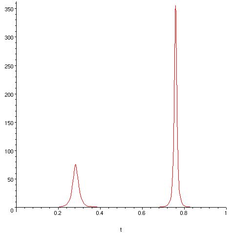 kappa is 1/27*abs(54+54*t^2-126*t)/(26-252*t+854*t^2-1176*t^3+565*t^4)^(3/2)
root of kappa between 0 and 1 is 7/6-1/6*13^(1/2)
======================================================================
Part B, Question 2
==================
First make functions that compute s(alpha,v) and d(alpha,v):
function w=s(alpha,v)
n=max(size(v,1),size(v,2));
w=zeros(size(v));
w(1)=v(1);
w(2:n-1)=v(2:n-1)+alpha*(v(1:n-2)-2*v(2:n-1)+v(3:n));
w(n)=v(n);
function w=d(alpha,v)
n=max(size(v,1),size(v,2));
w=zeros(size(v));
w(1)=v(2)-v(1);
w(2:n-1)=(v(3:n)+v(1:n-2))/2+alpha*(v(1:n-2)-2*v(2:n-1)+v(3:n));
w(n)=v(n)-v(n-1);
a)need an auxiliary function which computes s(alpha,v)^2 for given v,alpha
function z=n2(alpha,v)
w=s(alpha,v);
z=w*w';
for solving the problem use
function alpha=newb(v)
alpha=fminsearch(@n2,[0],[],v);
hold on
plot(v,'b.')
plot(s(alpha,v),'r-')
hold off
Here is an example of the graphical output, where v is a randon vector of length 100:
kappa is 1/27*abs(54+54*t^2-126*t)/(26-252*t+854*t^2-1176*t^3+565*t^4)^(3/2)
root of kappa between 0 and 1 is 7/6-1/6*13^(1/2)
======================================================================
Part B, Question 2
==================
First make functions that compute s(alpha,v) and d(alpha,v):
function w=s(alpha,v)
n=max(size(v,1),size(v,2));
w=zeros(size(v));
w(1)=v(1);
w(2:n-1)=v(2:n-1)+alpha*(v(1:n-2)-2*v(2:n-1)+v(3:n));
w(n)=v(n);
function w=d(alpha,v)
n=max(size(v,1),size(v,2));
w=zeros(size(v));
w(1)=v(2)-v(1);
w(2:n-1)=(v(3:n)+v(1:n-2))/2+alpha*(v(1:n-2)-2*v(2:n-1)+v(3:n));
w(n)=v(n)-v(n-1);
a)need an auxiliary function which computes s(alpha,v)^2 for given v,alpha
function z=n2(alpha,v)
w=s(alpha,v);
z=w*w';
for solving the problem use
function alpha=newb(v)
alpha=fminsearch(@n2,[0],[],v);
hold on
plot(v,'b.')
plot(s(alpha,v),'r-')
hold off
Here is an example of the graphical output, where v is a randon vector of length 100:
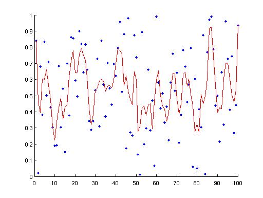 The procedure is a kind of averaging.
b)To do it coarsely in Maple is difficult. Instead, observe that
s(alpha,v) = v + alpha w for some suitable vector w
so we want to minimize alpha^2 w.w + 2 alpha w.v + v.v .
the minimum is where alpha = - w.v/w.w
c)very similar to a). auxiliary function
function z=n2(alpha,v)
w=s(alpha(3),d(alpha(2),s(alpha(1),v)));
z=w*w';
solution via
function alpha=newb(v)
alpha=fminsearch(@n2,[0;0;0],[],v);
======================================================================
Part B, Question 3
==================
a) with(LinearAlgebra);
findabc:=proc(p1,p2,p3)
local A,B,X,a,b,rs;
A:=<<2*op(1,p1),2*op(1,p2),2*op(1,p3)>|<2*op(2,p1),2*op(2,p2),2*op(2,p3)>|<1,1,1>>;
B:=<op(1,p1)^2+op(2,p1)^2,op(1,p2)^2+op(2,p2)^2,op(1,p3)^2+op(2,p3)^2>;
X:=LinearSolve(A,B);
a:=X[1]; b:=X[2]; rs:=X[3]+a^2+b^2;
return( (x-a)^2+(y-b)^2=rs );
end proc;
for example, findabc([2,2],[2,0],[0,2]) gives (x-1)^2+(y-1)^2=2
b) chk4:=proc(p1,p2,p3,p4)
local e1;
e1:=subs(x=op(1,p4),y=op(2,p4),findabc(p1,p2,p3));
if abs(evalf( op(1,e1)-op(2,e1) )) < 0.001 then return(1) else return(0) end if;
end proc;
======================================================================
Part B, Question 4
==================
Since M(s,t) is a symmetric matrix, it has real eigenvalues, and
eig returns them in increasing order. So all it is necessary to do
is make an m-file newb.m with contents
function z=newb(s)
M=[s(1) 2 s(2) 1; 2 -1 4 3; s(2) 4 s(1) 2; 1 3 2 4];
v=eig(M);
z=(v(1)+4)^2+(v(2)+2)^2+(v(3)-2)^2+(v(4)-4)^2;
and then do
[a b]=fminsearch( @newb, [0;0] )
to get a=[-0.8880 ; 1.2521] (values of s and t at the minimum)
b=17.3631 (minimum value of f(s,t)
For the second part make a function with contents
function z=newb(s)
M=[s(1) 2 s(2) 1; 2 -1 4 3; s(2) 4 s(1) 2; 1 3 2 4];
v=poly(M);
a1=v(1)*(-4)^4+v(2)*(-4)^3+v(3)*(-4)^2+v(4)*(-4)+v(5);
a2=v(1)*(-2)^4+v(2)*(-2)^3+v(3)*(-2)^2+v(4)*(-2)+v(5);
a3=v(1)*(2)^4 +v(2)*(2)^3 +v(3)*(2)^2 +v(4)*(2) +v(5);
a4=v(1)*(4)^4 +v(2)*(4)^3 +v(3)*(4)^2 +v(4)*(4) +v(5);
z=a1^2+a2^2+a3^2+a4^2;
NOTE: there is a shortcut to the linea a1=.. ,a2=... etc
can do a1=polyval(v,-4), a2=polyval(v,-2) etc.
but I do not think we learnt this command.
and then do
[a b]=fminsearch(@newb,[0;0])
to get a =[3.1156 ; 4.0692] (values of s and t at the minimum)
b =9.4960e+04 (minimum value of g(s,t)
======================================================================
The procedure is a kind of averaging.
b)To do it coarsely in Maple is difficult. Instead, observe that
s(alpha,v) = v + alpha w for some suitable vector w
so we want to minimize alpha^2 w.w + 2 alpha w.v + v.v .
the minimum is where alpha = - w.v/w.w
c)very similar to a). auxiliary function
function z=n2(alpha,v)
w=s(alpha(3),d(alpha(2),s(alpha(1),v)));
z=w*w';
solution via
function alpha=newb(v)
alpha=fminsearch(@n2,[0;0;0],[],v);
======================================================================
Part B, Question 3
==================
a) with(LinearAlgebra);
findabc:=proc(p1,p2,p3)
local A,B,X,a,b,rs;
A:=<<2*op(1,p1),2*op(1,p2),2*op(1,p3)>|<2*op(2,p1),2*op(2,p2),2*op(2,p3)>|<1,1,1>>;
B:=<op(1,p1)^2+op(2,p1)^2,op(1,p2)^2+op(2,p2)^2,op(1,p3)^2+op(2,p3)^2>;
X:=LinearSolve(A,B);
a:=X[1]; b:=X[2]; rs:=X[3]+a^2+b^2;
return( (x-a)^2+(y-b)^2=rs );
end proc;
for example, findabc([2,2],[2,0],[0,2]) gives (x-1)^2+(y-1)^2=2
b) chk4:=proc(p1,p2,p3,p4)
local e1;
e1:=subs(x=op(1,p4),y=op(2,p4),findabc(p1,p2,p3));
if abs(evalf( op(1,e1)-op(2,e1) )) < 0.001 then return(1) else return(0) end if;
end proc;
======================================================================
Part B, Question 4
==================
Since M(s,t) is a symmetric matrix, it has real eigenvalues, and
eig returns them in increasing order. So all it is necessary to do
is make an m-file newb.m with contents
function z=newb(s)
M=[s(1) 2 s(2) 1; 2 -1 4 3; s(2) 4 s(1) 2; 1 3 2 4];
v=eig(M);
z=(v(1)+4)^2+(v(2)+2)^2+(v(3)-2)^2+(v(4)-4)^2;
and then do
[a b]=fminsearch( @newb, [0;0] )
to get a=[-0.8880 ; 1.2521] (values of s and t at the minimum)
b=17.3631 (minimum value of f(s,t)
For the second part make a function with contents
function z=newb(s)
M=[s(1) 2 s(2) 1; 2 -1 4 3; s(2) 4 s(1) 2; 1 3 2 4];
v=poly(M);
a1=v(1)*(-4)^4+v(2)*(-4)^3+v(3)*(-4)^2+v(4)*(-4)+v(5);
a2=v(1)*(-2)^4+v(2)*(-2)^3+v(3)*(-2)^2+v(4)*(-2)+v(5);
a3=v(1)*(2)^4 +v(2)*(2)^3 +v(3)*(2)^2 +v(4)*(2) +v(5);
a4=v(1)*(4)^4 +v(2)*(4)^3 +v(3)*(4)^2 +v(4)*(4) +v(5);
z=a1^2+a2^2+a3^2+a4^2;
NOTE: there is a shortcut to the linea a1=.. ,a2=... etc
can do a1=polyval(v,-4), a2=polyval(v,-2) etc.
but I do not think we learnt this command.
and then do
[a b]=fminsearch(@newb,[0;0])
to get a =[3.1156 ; 4.0692] (values of s and t at the minimum)
b =9.4960e+04 (minimum value of g(s,t)
======================================================================
Back to course homepage
Back to my main teaching page
Back to my main page