Exam solutions, Moed Aleph, 5768 (Thursday group)
These are only notes, not full answers.
All the questions can be answered in many ways!
Especially the ones in part B.
==============================================================================
SECTION A, QUESTION 1
=====================
f1:=x^3-4*x^2-25*x+28;
f2:=x^3-3*x^2+4*x-12;
for roots do
solve(f1=0,x);
if that does not give satisfactory answers try
fsolve(f1=0,x);
for asymptotes do
solve(f2=0,x);
if that does not give satisfactory answers try
fsolve(f2=0,x);
for critical points do:
solve( diff(f1,x)*f2=diff(f2,x)*f1, x);
if that does not give satisfactory answers try
fsolve( diff(f1,x)*f2=diff(f2,x)*f1, x);
(note this gives only the real roots, which is what we want)
==============================================================================
SECTION A, QUESTION 2
=====================
function [a b]=findev(x)
M:=[1 3 -4;2 2 -2;x 7 -1];
[a b]=eigs(M);
==============================================================================
SECTION A, QUESTION 3
=====================
A is a matrix with 2 rows and 201 columns.
In the second of the four lines of code the first row of A is set to contain
the numbers from -1 to 1 in jumps of 0.01, and each entry of the second row
is cos(pi x/2) where x is the corresponding entry in the first row.
In the third of the four lines of code random numbers between -0.1 and 0.1
are added to each entry of A. So the relationship between entries in the
second and first rows is no longer true, but is approximately true.
In the fourth of the four lines two graphs are plotted: the blue line
is the true graph of cos(pi x/2), the red points are the columns of A
(treating the 1st row as the "x" coordinate and the 2nd row as the "y").
==============================================================================
SECTION A, QUESTION 4
=====================
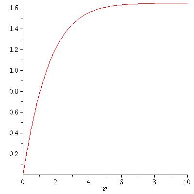
z1:=p->int(x/(exp(x)-1),x=0..p);
plot(z1(p),p=0..10);
Here's what you get:
 ==============================================================================
SECTION A, QUESTION 5
=====================
First a function to compute f as a function of x and t:
f.m
---
function y=f(x,t)
y=exp(-sin(x)/(1+x+t*x^2));
Now a function to find the minimum as a function of t:
fmin.m
------
function y=fmin(t);
y=fminsearch(@f,0,[],t);
This only works for a scalar t, let us make it work for a vector t:
fmin2.m
-------
function y=f2min(t);
y=zeros(size(t));
for i=1:size(t,1)
for j=1:size(t,2)
[v y(i,j)]=fminsearch(@f,0,[],t(i,j));
end
end
Now in the command line you can write
t=[1:0.04:5];
plot(t,fmin2(t))
==============================================================================
SECTION B, QUESTION 1
=====================
(a)
hints for understanding the procedure that follows:
x1y1 is [x1,y1]
x2y2 is [x2,y2]
abg is [alpha,beta,gamma]
checkside:=proc( x1y1, x2y2, abg )
local x1,y1,x2,y2,alpha,beta,gamma;
alpha:=op(1,abg); beta:=op(2,abg); gamma:=op(3,abg);
x1:=op(1,x1y1); y1:=op(2,x1y1);
x2:=op(1,x2y2); y2:=op(2,x2y2);
if (alpha*x1+beta*y1+gamma)*(alpha*x2+beta*y2+gamma)>0 then
return(true)
else return(false)
end if;
end proc;
(b)
hints for understanding the next part:
abg12 is the [alpha,beta,gamma] for the line joining x1y1 to x2y2
abg23 is the [alpha,beta,gamma] for the line joining x2y2 to x2y3
abg31 is the [alpha,beta,gamma] for the line joining x3y3 to x1y1
checktri:=proc(x1y1,x2y2,x3y3,xy)
local a,g,abg12, abg23, abg31;
if op(1,x1y1)=op(1,x2y2) then
abg12:=[1,0,-op(1,x1y1)];
else
a:=-(op(2,x2y2)-op(2,x1y1))/(op(1,x2y2)-op(1,x1y1));
g:=(op(1,x1y1)*op(2,x2y2)-op(1,x2y2)*op(2,x1y1))/(op(1,x2y2)-op(1,x1y1));
abg12:=[a,1,g];
end if;
if op(1,x3y3)=op(1,x2y2) then
abg23:=[1,0,-op(1,x3y3)];
else
a:=-(op(2,x2y2)-op(2,x3y3))/(op(1,x2y2)-op(1,x3y3));
g:=(op(1,x3y3)*op(2,x2y2)-op(1,x2y2)*op(2,x3y3))/(op(1,x2y2)-op(1,x3y3));
abg23:=[a,1,g];
end if;
if op(1,x1y1)=op(1,x3y3) then
abg31:=[1,0,-op(1,x1y1)];
else
a:=-(op(2,x3y3)-op(2,x1y1))/(op(1,x3y3)-op(1,x1y1));
g:=(op(1,x1y1)*op(2,x3y3)-op(1,x3y3)*op(2,x1y1))/(op(1,x3y3)-op(1,x1y1));
abg31:=[a,1,g];
end if;
if checkside(x3y3,xy,abg12) and checkside(x1y1,xy,abg23) and checkside(x2y2,xy,abg31) then
return(true);
else
return(false);
end if;
end proc;
==============================================================================
SECTION B, QUESTION 2
=====================
(a)
function y=findxminmax(a)
% a is the input vector
% y=[xmin xmax] is the output vector
r=roots(a);
realroots=[];
for i=1:size(r,1)
if imag(r(i))==0
realroots=[realroots;r(i)];
end;
end;
if size(realroots,1)==0
y=[0 0];
else
y=[min(realroots) max(realroots)]
end;
(b)
function y=findints(b,xmin,xmax)
% b,xmin,xmax are the inputs, as in the questionl; b a column vector
% y is a list of the form [ y1 y2
% y3 y4
% ...... ] each row an interval on which b\ge 4
% first find where b=4
c=b;
n=size(b,1);
c(n)=c(n)-4; % want to solve b=4
r=roots(c)
% extract the real roots in the ranges desired
goodroots=[xmin-1;xmax+1];
for ii=1:size(r,1)
if imag(r(ii))==0 & r(ii)>xmin-1 & r(ii)<xmax-1
goodroots=[goodroots;r(ii)];
end;
end;
% sort them out
g2=sort(goodroots)
% find the relevant intervals
y=[];
for ii=1:(size(g2,1)-1)
x=(g2(ii)+g2(ii+1))/2;
if polyval(b,x)>=4
y=[y;[g2(ii),g2(ii+1)]]
end;
end;
(c)
function makedr(a,b)
xs=findxminmax(a)
xmin=xs(1);
xmax=xs(2);
y=findints(b,xmin,xmax)
hold on
if size(y,1)==0 % draw on the whole interval
h=((xmax+1)-(xmin-1))/200;
x=xmin-1+[0:200]*h;
plot(x,polyval(a,x).*exp(polyval(b,x)))
else % draw on pieces of the interval
if y(1,1)>xmin-1
h=(y(1,1)-(xmin-1))/200;
x=xmin-1+[0:200]*h;
plot(x,polyval(a,x).*exp(polyval(b,x)))
end
for i=1:(size(y,1)-1)
h=(y(i+1,1)-y(i,2))/200;
x=y(i,2)+[0:200]*h;
plot(x,polyval(a,x).*exp(polyval(b,x)))
end
if y(size(y,1),2)<xmax+1
h=((xmax+1)-y(size(y,1),2))/200;
x=y(size(y,1),2)+[0:200]*h;
plot(x,polyval(a,x).*exp(polyval(b,x)))
end
end
==============================================================================
SECTION B, QUESTION 3
=====================
(a) Use 2 functions (it is possible just to use the quadratic formula for r)
f1.m
----
function y=f1(r,theta)
y=r^2*(cos(theta)^2+3*sin(theta)^2-2*cos(theta)*sin(theta))-r*(cos(theta)-4*sin(theta))-25;
f2.m
----
function r=f2(theta)
r=fzero(@f1,3,[],theta);
(b)
f3.m
----
function A=f3(theta)
% theta is the vector of 3 angles
r1=f2(theta(1));
r2=f2(theta(2));
r3=f2(theta(3));
% find the area
x1=r1*cos(theta1);
y1=r1*sin(theta1);
x2=r2*cos(theta2);
y2=r2*sin(theta2);
x3=r3*cos(theta3);
y3=r3*sin(theta3);
A=abs( (y3-y1)*(x2-x1) - (y2-y1)*(x3-x1) )/2
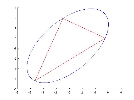
(c)
*** first need to redefine f3 to compute the negative of the area! ***
then the maximal area is obtained by
[ths S]:=fminsearch(f3,[0,2,4])
A=-S
the maximal area comes out about 24.2, but there are various different
values of the angles that give this.
here are a set of commands that draw the result:
f4.m
----
th=[0:0.02:7];
r=zeros(size(th));
for i=1:size(th,2)
r(i)=f2(th(i));
end
hold on
plot(r.*cos(th),r.*sin(th),'b')
[ths S]=fminsearch(@f3,[0,2,4]);
ths
A=-S
rs(1)=f2(ths(1));
rs(2)=f2(ths(2));
rs(3)=f2(ths(3));
plot([rs.*cos(ths),rs.*cos(ths)],[rs.*sin(ths),rs.*sin(ths)],'r')
==============================================================================
SECTION A, QUESTION 5
=====================
First a function to compute f as a function of x and t:
f.m
---
function y=f(x,t)
y=exp(-sin(x)/(1+x+t*x^2));
Now a function to find the minimum as a function of t:
fmin.m
------
function y=fmin(t);
y=fminsearch(@f,0,[],t);
This only works for a scalar t, let us make it work for a vector t:
fmin2.m
-------
function y=f2min(t);
y=zeros(size(t));
for i=1:size(t,1)
for j=1:size(t,2)
[v y(i,j)]=fminsearch(@f,0,[],t(i,j));
end
end
Now in the command line you can write
t=[1:0.04:5];
plot(t,fmin2(t))
==============================================================================
SECTION B, QUESTION 1
=====================
(a)
hints for understanding the procedure that follows:
x1y1 is [x1,y1]
x2y2 is [x2,y2]
abg is [alpha,beta,gamma]
checkside:=proc( x1y1, x2y2, abg )
local x1,y1,x2,y2,alpha,beta,gamma;
alpha:=op(1,abg); beta:=op(2,abg); gamma:=op(3,abg);
x1:=op(1,x1y1); y1:=op(2,x1y1);
x2:=op(1,x2y2); y2:=op(2,x2y2);
if (alpha*x1+beta*y1+gamma)*(alpha*x2+beta*y2+gamma)>0 then
return(true)
else return(false)
end if;
end proc;
(b)
hints for understanding the next part:
abg12 is the [alpha,beta,gamma] for the line joining x1y1 to x2y2
abg23 is the [alpha,beta,gamma] for the line joining x2y2 to x2y3
abg31 is the [alpha,beta,gamma] for the line joining x3y3 to x1y1
checktri:=proc(x1y1,x2y2,x3y3,xy)
local a,g,abg12, abg23, abg31;
if op(1,x1y1)=op(1,x2y2) then
abg12:=[1,0,-op(1,x1y1)];
else
a:=-(op(2,x2y2)-op(2,x1y1))/(op(1,x2y2)-op(1,x1y1));
g:=(op(1,x1y1)*op(2,x2y2)-op(1,x2y2)*op(2,x1y1))/(op(1,x2y2)-op(1,x1y1));
abg12:=[a,1,g];
end if;
if op(1,x3y3)=op(1,x2y2) then
abg23:=[1,0,-op(1,x3y3)];
else
a:=-(op(2,x2y2)-op(2,x3y3))/(op(1,x2y2)-op(1,x3y3));
g:=(op(1,x3y3)*op(2,x2y2)-op(1,x2y2)*op(2,x3y3))/(op(1,x2y2)-op(1,x3y3));
abg23:=[a,1,g];
end if;
if op(1,x1y1)=op(1,x3y3) then
abg31:=[1,0,-op(1,x1y1)];
else
a:=-(op(2,x3y3)-op(2,x1y1))/(op(1,x3y3)-op(1,x1y1));
g:=(op(1,x1y1)*op(2,x3y3)-op(1,x3y3)*op(2,x1y1))/(op(1,x3y3)-op(1,x1y1));
abg31:=[a,1,g];
end if;
if checkside(x3y3,xy,abg12) and checkside(x1y1,xy,abg23) and checkside(x2y2,xy,abg31) then
return(true);
else
return(false);
end if;
end proc;
==============================================================================
SECTION B, QUESTION 2
=====================
(a)
function y=findxminmax(a)
% a is the input vector
% y=[xmin xmax] is the output vector
r=roots(a);
realroots=[];
for i=1:size(r,1)
if imag(r(i))==0
realroots=[realroots;r(i)];
end;
end;
if size(realroots,1)==0
y=[0 0];
else
y=[min(realroots) max(realroots)]
end;
(b)
function y=findints(b,xmin,xmax)
% b,xmin,xmax are the inputs, as in the questionl; b a column vector
% y is a list of the form [ y1 y2
% y3 y4
% ...... ] each row an interval on which b\ge 4
% first find where b=4
c=b;
n=size(b,1);
c(n)=c(n)-4; % want to solve b=4
r=roots(c)
% extract the real roots in the ranges desired
goodroots=[xmin-1;xmax+1];
for ii=1:size(r,1)
if imag(r(ii))==0 & r(ii)>xmin-1 & r(ii)<xmax-1
goodroots=[goodroots;r(ii)];
end;
end;
% sort them out
g2=sort(goodroots)
% find the relevant intervals
y=[];
for ii=1:(size(g2,1)-1)
x=(g2(ii)+g2(ii+1))/2;
if polyval(b,x)>=4
y=[y;[g2(ii),g2(ii+1)]]
end;
end;
(c)
function makedr(a,b)
xs=findxminmax(a)
xmin=xs(1);
xmax=xs(2);
y=findints(b,xmin,xmax)
hold on
if size(y,1)==0 % draw on the whole interval
h=((xmax+1)-(xmin-1))/200;
x=xmin-1+[0:200]*h;
plot(x,polyval(a,x).*exp(polyval(b,x)))
else % draw on pieces of the interval
if y(1,1)>xmin-1
h=(y(1,1)-(xmin-1))/200;
x=xmin-1+[0:200]*h;
plot(x,polyval(a,x).*exp(polyval(b,x)))
end
for i=1:(size(y,1)-1)
h=(y(i+1,1)-y(i,2))/200;
x=y(i,2)+[0:200]*h;
plot(x,polyval(a,x).*exp(polyval(b,x)))
end
if y(size(y,1),2)<xmax+1
h=((xmax+1)-y(size(y,1),2))/200;
x=y(size(y,1),2)+[0:200]*h;
plot(x,polyval(a,x).*exp(polyval(b,x)))
end
end
==============================================================================
SECTION B, QUESTION 3
=====================
(a) Use 2 functions (it is possible just to use the quadratic formula for r)
f1.m
----
function y=f1(r,theta)
y=r^2*(cos(theta)^2+3*sin(theta)^2-2*cos(theta)*sin(theta))-r*(cos(theta)-4*sin(theta))-25;
f2.m
----
function r=f2(theta)
r=fzero(@f1,3,[],theta);
(b)
f3.m
----
function A=f3(theta)
% theta is the vector of 3 angles
r1=f2(theta(1));
r2=f2(theta(2));
r3=f2(theta(3));
% find the area
x1=r1*cos(theta1);
y1=r1*sin(theta1);
x2=r2*cos(theta2);
y2=r2*sin(theta2);
x3=r3*cos(theta3);
y3=r3*sin(theta3);
A=abs( (y3-y1)*(x2-x1) - (y2-y1)*(x3-x1) )/2
(c)
*** first need to redefine f3 to compute the negative of the area! ***
then the maximal area is obtained by
[ths S]:=fminsearch(f3,[0,2,4])
A=-S
the maximal area comes out about 24.2, but there are various different
values of the angles that give this.
here are a set of commands that draw the result:
f4.m
----
th=[0:0.02:7];
r=zeros(size(th));
for i=1:size(th,2)
r(i)=f2(th(i));
end
hold on
plot(r.*cos(th),r.*sin(th),'b')
[ths S]=fminsearch(@f3,[0,2,4]);
ths
A=-S
rs(1)=f2(ths(1));
rs(2)=f2(ths(2));
rs(3)=f2(ths(3));
plot([rs.*cos(ths),rs.*cos(ths)],[rs.*sin(ths),rs.*sin(ths)],'r')
 ==============================================================================
SECTION B, QUESTION 4
======================
(a)
If the determinant of M is 0 for all s, then the 3 last columns must be linearly
dependent. Call them c2,c3,c4 - it is then clear that c4 = 2 c3 - c2. Now we try
to express the first column (c1) as a linear sum of c2 and c3. We have 3c2 - 2c3
= [ -1 1 2 3]^T . Thus when s is NOT -1, the rank is 3 and the answer Maple gives
is correct. But when s=-1, the rank is 2, and Maple has made an error.
(b)
Suppose the matrix is M, which depends on s,t.
To see if there is a double eigenvalue 0: we need the first two terms
in the characteristic polynomial to be zero. Find when this happens by:
c:=CharacteristicPolynomial(M,x);
solve( {coeff(c,x,0)=0,coeff(c,x,1)=0} , {s,t} );
To see if the column space is 2 dimensional: Using "ColumnSpace" or "Rank" will
not work, as we saw in part (a) that Maple makes assumptions. As we shall see,
note also that in general there will be no solution to this problem (as it
requires 3 conditions on the 2 parameters s,t). Here is one approach:
First find s as a function of t by requiring the determinant to be zero:
d:=Determinant(M);
s1:=solve( d=0, s);
M1:=subs(s=s1,M);
If the column space is two dimensional we should be able to build the 1st
and 2nd column out of the third and fourth. So can try something like this
v:=M[1..4,1]-a*M[1..4,3]-b*M[1..4,4];
solve( {v[1]=0,v[2]=0} , {a,b} );
assigm(%)
t1:=solve( v[3]=0, t);
subs(t=t1,v[4]);
if you get zero at the end, then t1 is the value of t and
subs(t=t1,s1);
gives the value of s. Any value of t you get can also be checked by
M2:=subs(t=t1,M1);
ColumnSpace(M2);
==============================================================================
==============================================================================
SECTION B, QUESTION 4
======================
(a)
If the determinant of M is 0 for all s, then the 3 last columns must be linearly
dependent. Call them c2,c3,c4 - it is then clear that c4 = 2 c3 - c2. Now we try
to express the first column (c1) as a linear sum of c2 and c3. We have 3c2 - 2c3
= [ -1 1 2 3]^T . Thus when s is NOT -1, the rank is 3 and the answer Maple gives
is correct. But when s=-1, the rank is 2, and Maple has made an error.
(b)
Suppose the matrix is M, which depends on s,t.
To see if there is a double eigenvalue 0: we need the first two terms
in the characteristic polynomial to be zero. Find when this happens by:
c:=CharacteristicPolynomial(M,x);
solve( {coeff(c,x,0)=0,coeff(c,x,1)=0} , {s,t} );
To see if the column space is 2 dimensional: Using "ColumnSpace" or "Rank" will
not work, as we saw in part (a) that Maple makes assumptions. As we shall see,
note also that in general there will be no solution to this problem (as it
requires 3 conditions on the 2 parameters s,t). Here is one approach:
First find s as a function of t by requiring the determinant to be zero:
d:=Determinant(M);
s1:=solve( d=0, s);
M1:=subs(s=s1,M);
If the column space is two dimensional we should be able to build the 1st
and 2nd column out of the third and fourth. So can try something like this
v:=M[1..4,1]-a*M[1..4,3]-b*M[1..4,4];
solve( {v[1]=0,v[2]=0} , {a,b} );
assigm(%)
t1:=solve( v[3]=0, t);
subs(t=t1,v[4]);
if you get zero at the end, then t1 is the value of t and
subs(t=t1,s1);
gives the value of s. Any value of t you get can also be checked by
M2:=subs(t=t1,M1);
ColumnSpace(M2);
==============================================================================
Back to course homepage
Back to my teaching homepage
Back to my homepage