                           ===========
                           S c i l a b
                           ===========


                          scilab-2.6
                  Copyright (C) 1989-2001 INRIA


Startup execution:
  loading initial environment

-->
The Scilab window has various pull-down menus you can explore. You should sometime look at the demos and also the on-line help. To obtain help on a particular command or subject, say the subject "matrix", type "apropos matrix".
Let's start by entering a 4x4 matrix and calling it A:
--> A=[16 3 2 15; 15 10 11 8; 9 6 7 12; 4 15 14 1]
 A =

!    16.    3.     2.    15. !
!    15.    10.    11.   8   !
!    9.     6.     7.    12. !
!    4.     15.    14.   1.  !

-->
Let's ask Scilab for its transpose:
-->A'
 ans  =

!   16.    15.    9.     4.  !
!   3.     10.    6.     15. !
!   2.     11.    7.     14. !
!   15.    8.     12.    1.  !

-->
We will now enter a 4-dimensional row vector, and try to form the products bA and Ab:
-->b = [1.4 5.23 1.22 -1.1]
 b  =

!   1.4    5.23    1.22  - 1.1 !

-->b*A
 ans  =

!   107.43    47.32    53.47    76.38 !

-->A*b
    !--error    10
inconsistent multiplication
Of course, we can multiply a 4-dimensional row vector on the right by a 4x4 matrix, but not on the left. If we enter a 4-dimensional column vector, we can left multiply, but not right multiply:
-->b = [1.4; 5.23; 1.22; -1.1]
 b  =

!   1.4  !
!   5.23 !
!   1.22 !
! - 1.1  !

-->A*b
 ans  =

!   24.03  !
!   77.92  !
!   39.32  !
!   100.03 !

-->b*A
    !--error    10
inconsistent multiplication
Suppose we want to solve the equation Av=b. Formally the solution is v=A-1b, so we need to divide b by A on the left. We'll do this now, and then check by computing Av and Av-b.
-->v=A\b
 v  =

!   0.5069868 !
! - 1.4192053 !
!   1.3214238 !
! - 0.3398013 !

-->A*v
 ans  =

!   1.4  !
!   5.23 !
!   1.22 !
! - 1.1  !

-->A*v-b
 ans  =

   1.0E-14 *

!   0.0444089 !
!   0.1776357 !
!   0.0444089 !
!   0.0444089 !
Note that the last answer is not exactly zero. There is rounding error. The rounding error is very small; Scilab works to about 16 figure accuracy, but does not usually print answers using such precision.
If we make b a row vector again, we can try to solve b=wA. The solution is w=bA-1, so we need to divide b on the right by A:
-->b = [1.4 5.23 1.22 -1.1]
 b  =

!   1.4    5.23    1.22  - 1.1 !

-->w=b/A
 w  =

!   1.1282923  - 0.7273415  - 1.1046168    1.0497493 !

-->w*A
 ans  =

!   1.4    5.23    1.22  - 1.1 !

-->w*A-b
 ans  =

   1.0E-15 *

!   0.6661338    0.  - 0.4440892    0.6661338 !
Here's a shortcut to produce a row vector with the entries 0,1,2,...,10:
-->t=0:10
 t  =

!   0.    1.    2.    3.    4.    5.    6.    7.    8.    9.    10. !

-->
If we want a row vector with entries 0,0.1,0.2,...9.9,10.0 we can get it with
-->t=0:0.1:10;

-->
Note I have supressed output by finishing the line with a ;
Most functions in Scilab work componentwise on matrices. So we can do
-->y=sin(t);

-->
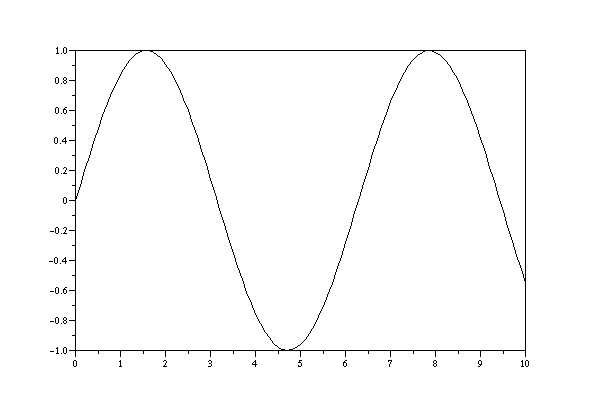
and the supressed output will be 101-dimensional vector with the values of sin(t) in for t = 0,0.1,0.2,..10.0. We can now get a graph of sin(t) by plotting y against t:
-->plot(t,y)

-->
The output appears in another window, and looks like this:

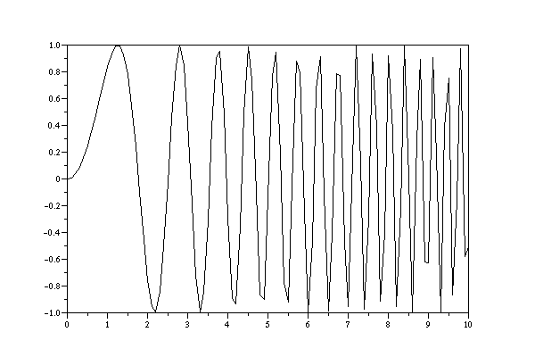
What if I want the graph of sin(t2)? First try:
-->z=sin(t*t)
          !--error    10
inconsistent multiplication


-->
t is a row vector and so this tried to multiply two vectors, which fails. We need "component-wise multiplication" using .*:
-->z=sin(t.*t);

-->plot(t,z)

-->
The result is:

In the demos you can find more details on basic graphics.
Now, it is a pain to type input to Scilab after the prompt sign, particularly if the same or similar input is used several times. But in fact you can use files for input. These files sit in your working directory.
A=[ 16  3  2  15; 15  10  11  8;  9  6  7  12;  4 15  14  1]
b=[ 1.4; 5.23; 1.22;  -1.1]
v=A\b
The if in my Scilab session I type "exec input1" I get the following response:
-->exec input1

-->A=[ 16  3  2  15; 15  10  11  8;  9  6  7  12;  4 15  14  1]
 A  =

!   16.    3.     2.     15. !
!   15.    10.    11.    8.  !
!   9.     6.     7.     12. !
!   4.     15.    14.    1.  !

-->b=[ 1.4; 5.23; 1.22;  -1.1]
 b  =

!   1.4  !
!   5.23 !
!   1.22 !
! - 1.1  !

-->v=A\b
 v  =

!   0.5069868 !
! - 1.4192053 !
!   1.3214238 !
! - 0.3398013 !


-->
Scilab reads and executes all commands in the file input1.
function a=func1(x)
a = (1-exp(x)*sin(x)+x^3) / (x*tan(x)+0.5)
endfunction
When I do "exec func1", Scilab reads in this function:
-->exec func1

-->function a=func1(x)
-->a = (1-exp(x)*sin(x)+x^3) / (x*tan(x)+0.5)
-->endfunction

-->
and now I can use it, for example:
-->func1(2)
 ans  =

  - 0.5894324

-->
If I want to read in the function but not print it out, it should be called with a ";", i.e. by typing "exec func1;".
Suppose we try to apply our new function to a vector:
-->func1([1 2])
 !--error    10
inconsistent multiplication
at line       2 of function func1                    called by :
func1([1 2])
We should have defined the operations in the function to be componentwise operations. So let's change the file to
function a=func1(x)
a= (1-exp(x).*sin(x)+x.^3) ./ (x.*tan(x)+0.5);
endfunction
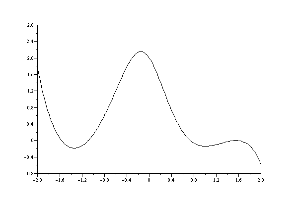
Suppose now that we want to find the roots of func1, i.e. the points x such that func1(x)=0. We do
-->exec func1;

-->x=-2:0.02:2;

-->plot(x,func1(x))
to get

One root is (I guess) between -1.6 and -1.5. Let's track it down by what is known as "interval bisection":
-->func1(-1.6)
 ans  =

    0.0533274

-->func1(-1.5)
 ans  =

  - 0.0994096

-->func1(-1.55)
 ans  =

  - 0.0334793

-->func1(-1.575)
 ans  =

    0.0072159

-->func1(-1.5625)
 ans  =

  - 0.0137958

-->func1(-1.56875)
 ans  =

  - 0.0034576

-->func1(-1.571875)
 ans  =

    0.0018371
Let's automate this procedure. The function below in the file bisec1 inputs a 2-vector a1 which is the initial interval that contains the root, and an integer n which is the number of times we want to bisect this interval:
function a2=bisec1(a1,n)

f=func1(a1);

for i=1:n
   mid=(a1(1)+a1(2))/2;
   midf=func1(mid);
   if (midf*f(1)>0)
        a1(1)=mid;
        f(1)=midf;
     else
        a1(2)=mid;
        f(2)=midf;
   end
end

a2=a1;
endfunction
Lots of new things in this function: calling a vector's components, the for loop syntax (note the "end"), the if syntax (note the "end").
Problems with this function: does it work if you land exactly on the zero? What other problems can you spot?
Here is a run of this program doing 30 more bisections.
-->exec bisec1;

-->bisec1([-1.6 -1.5],30)
 ans  =

! - 1.5707963  - 1.5707963 !

-->
The accuracy of the presentation is insufficient here. Here's how to fix it:
-->format(16)

-->bisec1([-1.6 -1.5],30)
 ans  =

! - 1.5707963268273  - 1.5707963267341 !

-->
Exercise: find the other roots visible on the graph, each to 12 figure accuracy.
For more information on scilab you should look at the official introduction