function C = t1(rho)

sigma=0.25;
X0=1;
Y0=0;
N=100;           % number of steps
M=10000;         % number of simulations
h=2/N;           % timestep

% make matrices to hold the answers
X=X0*ones(M,N+1);
Y=Y0*ones(M,N+1);

% make random numbers
Z1=randn(M,N);
Z2=randn(M,N);

% make correlated random numbers
W1=Z1;
W2=rho*Z1+sqrt(1-rho^2)*Z2;

%Euler Maruyama
for i=1:N
    X(:,i+1)=X(:,i)+h*Y(:,i)+sqrt(h)*sigma*W1(:,i);
    Y(:,i+1)=Y(:,i)-h*X(:,i)+sqrt(h)*sigma*W2(:,i);
end

a =X(:,N+1).^2+Y(:,N+1).^2;
C = [mean(a), std(a)/sqrt(M)];
Results: The first number is the answer, the second number is the stochastic error.
>> t1(0)

ans =

    1.2928    0.0076

>> t1(0.3)

ans =

    1.2899    0.0072

>> t1(-0.3)

ans =

    1.3000    0.0082
To make a plot .... this is not the best way, but it is simple and works:
rho=-1:0.02:1;
a=zeros(size(rho));
b=zeros(size(rho));
for i=1:length(rho)
    C=t1(rho(i));
    a(i)=C(1);
    b(i)=C(2);
end
figure(1)
plot(rho,a)
figure(2)
plot(rho,b)
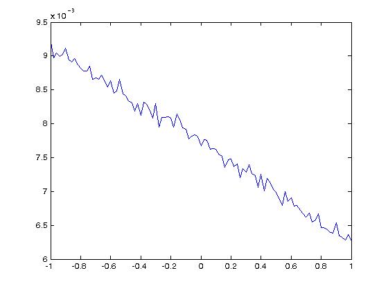
Here are the plots:


The plot of the value does not look very nice. In fact what we are seeing is that C does not depend on rho, just for each value there is a different stochastic error which gives the up-and-down effects. The second plot shows that the stochastic error is about 0.007, so we can expect results to go up-and-down by about 0.015 which is what we see.
I would have been better off using common random variables, but it actually is harder to interpret the results
% set all the parameters of the problem, and the numeric parameters
r=0.06;
sigma=0.2;
alpha=0.04;
S0=1;
T=1;
K=1;

N=100;
M=10000;
h=T/N;

% make prices with Euler-Maruyama
Z=randn(M,N);
S=S0*ones(M,N+1);
for i=1:N
    S(:,i+1)=S(:,i) + h*r*S(:,i)+(sigma*S(:,i)./(1+alpha*S(:,i).^2))*sqrt(h).*Z(:,i);
end

% values of the 3 options - putting in exp(-rT) factor
V1 = exp(-r*T)*max(S(:,N+1)-K,0) ;
V2 = exp(-r*T)*max(max(S,[],2)-K ,0) ;
V3 = exp(-r*T)*max(sum(S,2)/(N+1)-K,0) ;

[mean(V1),std(V1)/sqrt(M)]
[mean(V2),std(V2)/sqrt(M)]
[mean(V3),std(V3)/sqrt(M)]
The results:
ans =

    0.1078    0.0014


ans =

    0.1776    0.0015


ans =

    0.0589    0.0008
Does this make sense? Yes! A max option is worth more than a regular option because if detects the highest price, wherever it is in the time interval. In general a regular option is worth more than an asiatic option as on average the price increases over the time interval so on average the value at the end is higher than the average value. (Here I am using "average" in two senses - average over the time interval and average over different simulations.)
The stochastic error is about 1% for the regular option, so the M I took was big enough (just luck).
kappa=2;
lambda=2;
N=20;
M=2000;      % going to use Euler method - need stability - 1000 did not work
h=1/N;
k=1/M;
x=(0:N)*h;

u=zeros(M+1,N+1);
u(1,:) = x.^2;     % initial condition
u(:,N+1)=1;        % right hand boundary

for j=1:M         % the Euler loop
    u(j+1,2:N)=u(j,2:N) + kappa*k/h^2*(u(j,3:(N+1))-2*u(j,2:N)+u(j,1:(N-1))) - lambda*k*u(j,2:N) ;
    u(j+1,1) = 4/3*u(j+1,2)-1/3*u(j+1,3);     % this is to impose the boundary condition at the left hand side
end

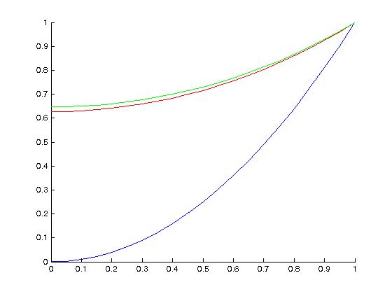
figure(1)   % plot at t=0, 0.5, 1
hold on
plot(x,u(1,:),'b');
plot(x,u(M/2+1,:),'r');
plot(x,u(M+1,:),'g');
hold off

u(M+1,1)              % value of u(0,1)
u(M+1,4*N/5+1)        % value of u(0.8,1)
Plot:

The numbers I go were 0.6474 and 0.8666. We tell these are accurate enough by running again with N=40 and M=8000 (stability means if we multiply N by 2, we must multiply M by 4). I got 0.6474 and 0.8665. So the accuracy was already good enough. If I take N=10 and M=500 I get 0.6475 and 0.8666. Even with N=5 and M=120 I could not get any reasonable error! There is a reason for this to be sure....
Back to main course page
Back to my main teaching page
Back to my home page