
%%%%%%%%%%%%%%%%%%%%%%%%%%%%%%%%%%%%%%%%%%%%%%%%%%%%%%%%%%%%%%%%%%%%%
r=0.1;
s=0.4;
S0=1.0;
K=1.1;
T=60/252;
N=600;
M=50000;
h = T/N;
Z = randn(M,N);

S  = S0*ones(M,N+1);

% make prices
for i=1:N
    S(:,i+1)  = S(:,i).*exp((r-s^2/2)*h + sqrt(h)*s*Z(:,i));
end

Smax  = max(S,[],2);
p = sum(Smax>K)/M
err = sqrt(p*(1-p)/M)
%%%%%%%%%%%%%%%%%%%%%%%%%%%%%%%%%%%%%%%%%%%%%%%%%%%%%%%%%%%%%%%%%%%%%
Can you explain the formula for the stochastic error?
Here is the same made to run for a range of values of K, with plots:
%%%%%%%%%%%%%%%%%%%%%%%%%%%%%%%%%%%%%%%%%%%%%%%%%%%%%%%%%%%%%%%%%%%%%
r=0.1;
s=0.4;
S0=1.0;
T=60/252;
N=600;
M=50000;
h = T/N;
Z = randn(M,N);

S  = S0*ones(M,N+1);

% make prices
for i=1:N
    S(:,i+1)  = S(:,i).*exp((r-s^2/2)*h + sqrt(h)*s*Z(:,i));
end

Smax  = max(S,[],2);

K = 0.95:0.002:1.6;
p = zeros(size(K));
err = zeros(size(K));

for i=1:length(K)
  p(i) = sum(Smax>K(i))/M;
  err(i) = sqrt(p(i)*(1-p(i))/M);
end

figure(1)
plot(K,p)
title('probability as a function of K')
xlabel('K')
ylabel('probability')
figure(2)
plot(K,err)
title('stochastic error as a function of K')
xlabel('K')
ylabel('stochastic error')
%%%%%%%%%%%%%%%%%%%%%%%%%%%%%%%%%%%%%%%%%%%%%%%%%%%%%%%%%%%%%%%%%%%%%
Here are the plots:

The probability is 1 if K is less than 1 and falls as K increases.
Part b: When K is large, most of the time the option return is zero. So in our simulation of the price (using the program from question 2) most runs are wasted, as they just give zero. For K=1.4 the probability of a positve return is less than 0.1, so 90% of the work is wasted. If we use random variables with a N(mu,1) distribution with mu>0 we will spend more time exploring the "interesting" region and have less wasted runs.
Part c: Here is a program that computes using N(mu,1) random numbers. There are 2 changes - the random numbers are chosen differently, and the return function has to be modified (the formula for this was proved in class). NOTE: this year I did not discuss how mu should change with N. But since in this program I keep N fixed at 600, we can ignore this issue.
%%%%%%%%%%%%%%%%%%%%%%%%%%%%%%%%%%%%%%%%%%%%%%%%%%%%%%%%%%%%%%%%%%%%%
r=0.1;
s=0.4;
S0=1.0;
T=60/252;
K=1.4;
N=600;
M=50000;
h = T/N;

% make the random numbers with a N(mu,1) distribution
mu = 0.1;
Z = mu+randn(M,N);

S  = S0*ones(M,N+1);

% make prices
for i=1:N
    S(:,i+1)  = S(:,i).*exp((r-s^2/2)*h + sqrt(h)*s*Z(:,i));
end

Smax  = max(S,[],2);
ret = exp(-r*T)*(Smax-K).*(Smax>K);
% modify the return to take into account the new distribution
%    formula was explained in class
retmod = ret .* exp(-mu*sum(Z,2))*exp(mu^2*N/2) ;
mean(retmod)
std(retmod)/sqrt(M)
%%%%%%%%%%%%%%%%%%%%%%%%%%%%%%%%%%%%%%%%%%%%%%%%%%%%%%%%%%%%%%%%%%%%%
Here are plots of the results obtained for values of mu from 0 to 0.16:
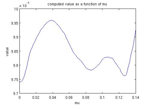

We are seeing a best value of mu at about 0.07, giving a value of the option as 0.00982 with an error of 0.0006. The plot of the values of the option varies (quite significantly) from run to run - but the plot of the stochastic error remains the same.
Part d: Absolutely no reason not to use this method to compute the Delta!! We will compare mu=0 and mu=0.07. Here is my program, I hope I got it all right:
%%%%%%%%%%%%%%%%%%%%%%%%%%%%%%%%%%%%%%%%%%%%%%%%%%%%%%%%%%%%%%%%%%%%%
r=0.1;
s=0.4;
S0=1.0;
T=60/252;
K=1.4;
N=600;
M=50000;
h = T/N;
eps = 0.0001;    % for computing the delta

% make the random numbers with a N(mu,1) distribution
mu = 0.07;
Z = mu+randn(M,N);

% make two matrices of prices
Splus  = (S0+eps)*ones(M,N+1);
Sminus = (S0-eps)*ones(M,N+1);

% make prices
for i=1:N
    Splus(:,i+1)  = Splus(:,i).*exp((r-s^2/2)*h + sqrt(h)*s*Z(:,i));
    Sminus(:,i+1)  = Sminus(:,i).*exp((r-s^2/2)*h + sqrt(h)*s*Z(:,i));
end

% make returns and modified returns
Splusmax  = max(Splus,[],2);
retplus = exp(-r*T)*(Splusmax-K).*(Splusmax>K);
retmodplus = retplus .* exp(-mu*sum(Z,2))*exp(mu^2*N/2) ;

Sminusmax  = max(Sminus,[],2);
retminus = exp(-r*T)*(Sminusmax-K).*(Sminusmax>K);
retmodminus = retminus .* exp(-mu*sum(Z,2))*exp(mu^2*N/2) ;

sens = (retmodplus - retmodminus)/(2*eps);
mean(sens)
std(sens)/sqrt(M)
%%%%%%%%%%%%%%%%%%%%%%%%%%%%%%%%%%%%%%%%%%%%%%%%%%%%%%%%%%%%%%%%%%%%%
With mu=0.007 I got typical answers of 0.125 with stochastic errors of 0.001. With mu=0 I got answers in the range 0.122 to 0.130 with stochastic errors of 0.002. Using importance sampling here has reduced the stochastic error by about 40% (it looks like 50% but I have rounded generously). This was for a value of K where "only" 90% of simulations were being wasted. For higher K the variance reduction would have been even more pronounced.
Back to main course page
Back to my main teaching page
Back to my home page