That is, it takes x=1/2 and does x=ax(1-x) N times, and at the end subtracts 1/2. If this gives zero, then there is a superstable Nth order periodic orbit.
Note the function works for input values of a that are vectors or matrices.
function y=log3(a,N)

y=zeros(size(a));

for i=1:size(a,1)
  for j=1:size(a,2)

    x=0.5;
    for k=1:N
	    x=a(i,j)*x*(1-x);
    end
    y(i,j)=x-0.5;

  end
end
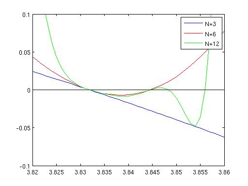
The first thing you should do with this is plot log3(a,3), log3(a,6) and log3(a,12) for a in the interval 3.82-3.86. This is what the results look like:
Of course any (superstable) period 3 orbit is a period 6 orbit etc. So all zeros of log3(a,3) are zeros of log3(a,6) are zeros of log3(a,12) etc. Once you have the plots you can use fzero carefully to get the desired roots of the necessary functions. Below there is a Matlab script that does everything - plots the plots, finds the roots etc. (and the a values are given as comments).
To do the same for N=24 and N=48 requires great care. The functions log3(a,24) and log3(a,48) behave quite wildly if you take a range of a that is too large. In the Matlab script below you can see appropriate ranges. The relevant plot looks like this:
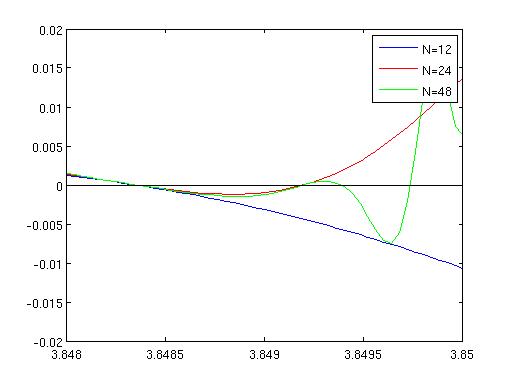
Once you have the plot, it is easy to pick out the zeros. See the script for all the details and the numbers.
a=3.82:0.001:3.86;
b1=log3(a,3);
b2=log3(a,6);
b3=log3(a,12);
figure(1)
plot(a,b1,'b',a,b2,'r',a,b3,'g',a,zeros(size(a)),'k')
xlim([3.82 3.86])
ylim([-0.1 0.1])
legend('N=3','N=6','N=12')

fzero(@(x) log3(x,3) , [3.825 3.835])   %  answer 3.831874
fzero(@(x) log3(x,6) , [3.844 3.846])   %  answer 3.844569
fzero(@(x) log3(x,12), [3.846 3.85])    %  answer 3.848345

a=3.848:0.00004:3.850;
b1=log3(a,12);
b2=log3(a,24);
b3=log3(a,48);
figure(2)
plot(a,b1,'b',a,b2,'r',a,b3,'g',a,zeros(size(a)),'k')
xlim([3.848 3.850])
ylim([-0.02 0.02])
legend('N=12','N=24','N=48')

fzero(@(x) log3(x,12) , [3.848  3.8485])   %  answer 3.848345
fzero(@(x) log3(x,24) , [3.849  3.8493])   %  answer 3.849198
fzero(@(x) log3(x,48) , [3.8493 3.8494])   %  answer 3.849383

% differences between the 5 a values:
% 0.012695
% 0.003776   (1/3.36 times previous)
% 0.000853   (1/4.43 times previous)
% 0.000185   (1/4.61 times previous)
The important thing to notice is that the difference between pairs of a values
drops by about 1/4 each time. In fact if we would continue the process we would see
the ratio tends to the The
Feigenbaum constant 4.669... You might also notice that the two plots above look exactly the same, only scaled. This is at the heart of Feigenbaum's renormalization theory.
Back to main course page
Back to my main teaching page
Back to my home page